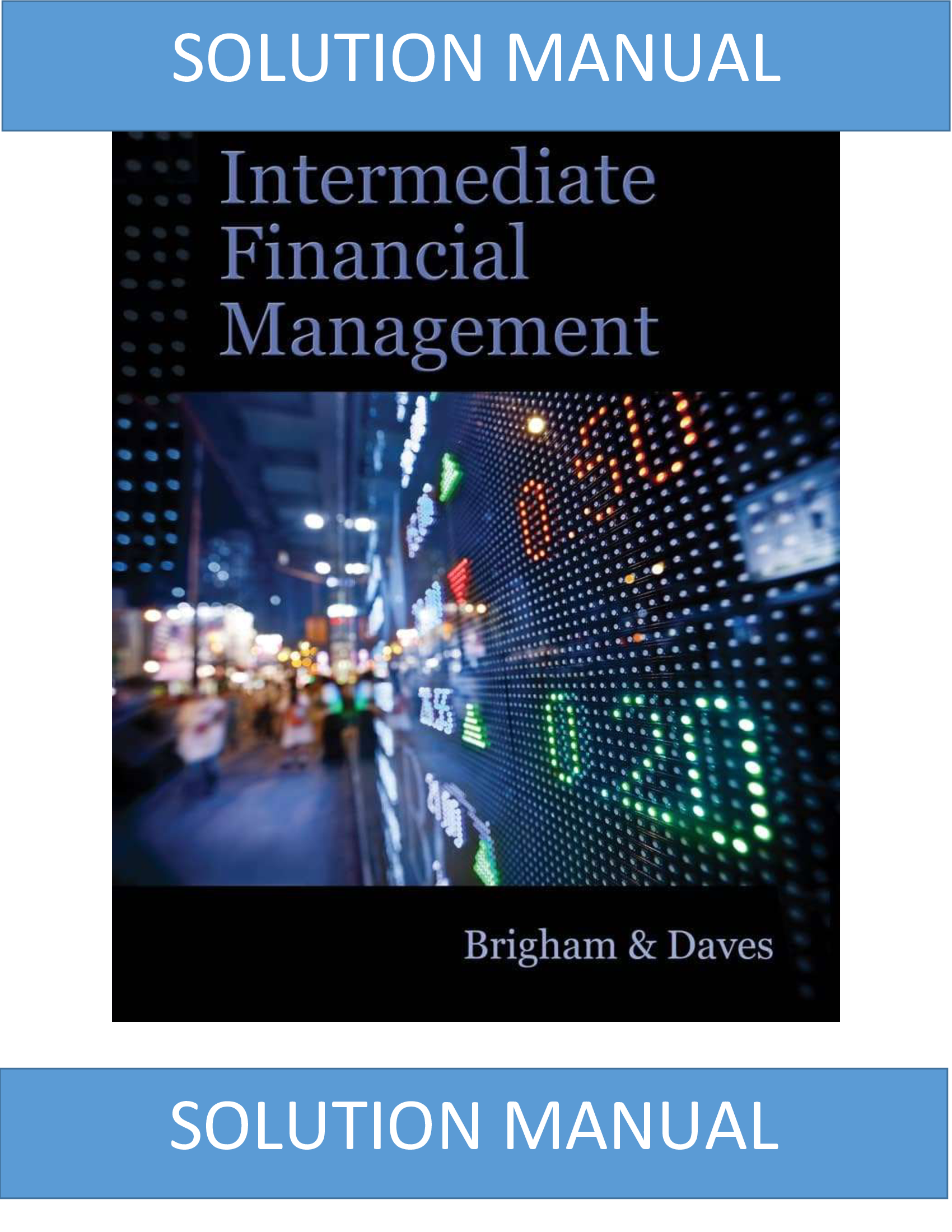
Solution Manual for Intermediate Financial Management, 11th Edition, Eugene F. Brigham Phillip R. Daves

Solution Manual for Intermediate Financial Management

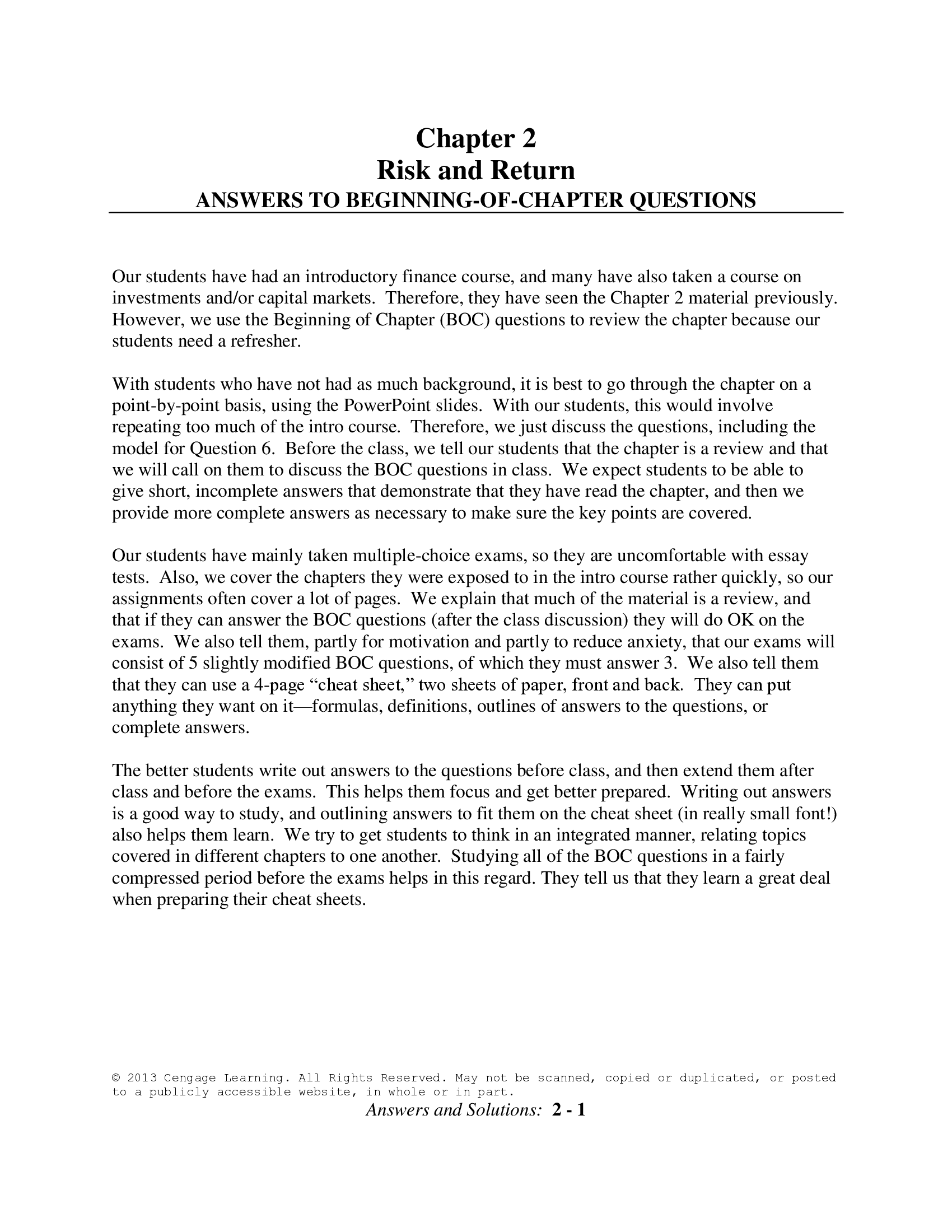
Chapter 2 Risk and Return

ANSWERS TO BEGINNING-OF-CHAPTER QUESTIONS      

Our students have had an introductory finance course, and many have also taken a course on investments and/or capital markets.  Therefore, they have seen the Chapter 2 material previously. However, we use the Beginning of Chapter (BOC) questions to review the chapter because our students need a refresher.

With students who have not had as much background, it is best to go through the chapter on a point-by-point basis, using the PowerPoint slides.  With our students, this would involve repeating too much of the intro course.  Therefore, we just discuss the questions, including the model for Question 6.  Before the class, we tell our students that the chapter is a review and that we will call on them to discuss the BOC questions in class.  We expect students to be able to give short, incomplete answers that demonstrate that they have read the chapter, and then we provide more complete answers as necessary to make sure the key points are covered.

Our students have mainly taken multiple-choice exams, so they are uncomfortable with essay tests.  Also, we cover the chapters they were exposed to in the intro course rather quickly, so our assignments often cover a lot of pages.  We explain that much of the material is a review, and that if they can answer the BOC questions (after the class discussion) they will do OK on the

exams.  We also tell them, partly for motivation and partly to reduce anxiety, that our exams will consist of 5 slightly modified BOC questions, of which they must answer 3.  We also tell them that they can use a 4-page “cheat sheet,” two sheets of paper, front and back.  They can put anything they want on it—formulas, definitions, outlines of answers to the questions, or complete answers.

The better students write out answers to the questions before class, and then extend them after class and before the exams.  This helps them focus and get better prepared.  Writing out answers is a good way to study, and outlining answers to fit them on the cheat sheet (in really small font!) also helps them learn.  We try to get students to think in an integrated manner, relating topics covered in different chapters to one another.  Studying all of the BOC questions in a fairly compressed period before the exams helps in this regard. They tell us that they learn a great deal when preparing their cheat sheets.

We initially expected really excellent exams, given that the students had the questions and could use cheat sheets.  Some of the exams were indeed excellent, but we were surprised and disappointed at the poor quality of many of the midterm exams.  Part of the problem is that our students were not used to taking essay exams.  Also, they would have done better if they had taken the exam after we covered cases (in the second half of the semester), where we apply the text material to real-world cases.  While both points are true, it’s also true that some students are just better than others.

The students who received low exam grades often asked us what they did wrong.  That’s often a hard question to answer regarding an essay exam.  What we ended up doing was make copies of the best 2 or 3 student answers to each exam question, and then when students came in to see why they did badly, we made them read the good answers before we talked with them.   95% of the time, they told us they understand why their grade was low, and they resolved to do better next time.  Finally, since our students are all graduating seniors, we graded rather easily.

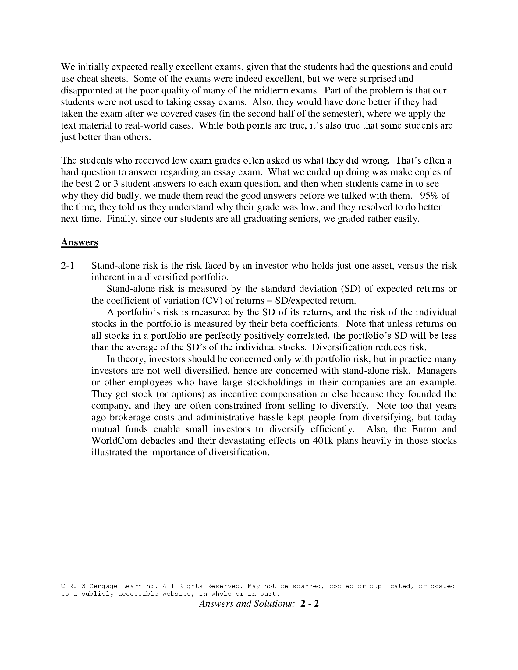
Answers

2-1      Stand-alone risk is the risk faced by an investor who holds just one asset, versus the risk inherent in a diversified portfolio.

Stand-alone risk is measured by the standard deviation (SD) of expected returns or the coefficient of variation (CV) of returns = SD/expected return.

A portfolio’s risk is measured by the SD of its returns, and the risk of the individual stocks in the portfolio is measured by their beta coefficients.  Note that unless returns on all stocks in a portfolio are perfectly positively correlated, the portfolio’s SD will be less than the average of the SD’s of the individual stocks. Diversification reduces risk.

In theory, investors should be concerned only with portfolio risk, but in practice many investors are not well diversified, hence are concerned with stand-alone risk.  Managers or other employees who have large stockholdings in their companies are an example. They get stock (or options) as incentive compensation or else because they founded the company, and they are often constrained from selling to diversify.  Note too that years ago brokerage costs and administrative hassle kept people from diversifying, but today mutual funds enable small investors to diversify efficiently.   Also, the Enron and WorldCom debacles and their devastating effects on 401k plans heavily in those stocks illustrated the importance of diversification.

2-2      Diversification can eliminate unsystematic risk, but market risk will remain.  See Figure

2-8 for a picture of what happens as stocks are added to a portfolio.  The graph shows that the risk of the portfolio as measured by its SD declines as more and more stocks are added.  This is the situation if randomly selected stocks are added, but if stocks in the same industry are added, the benefits of diversification will be lessened.

Conventional wisdom says that 40 to 50 stocks from a number of different industries is sufficient to eliminate most unsystematic risk, but in recent years the markets have become increasingly volatile, so now it takes somewhat more, perhaps 60 or 70.   Of course, the more stocks, the closer the portfolio will be to having zero unsystematic risk. Again, this assumes that stocks are randomly selected.   Note, however, that the more stocks the portfolio contains, the greater the administrative costs.  Mutual funds can help here.

Different diversified portfolios can have different amounts of risk.  First, if the portfolio concentrates on a given industry or sector (as sector mutual funds do), then the portfolio will not be well diversified even if it contains 100 stocks.  Second, the betas of the individual stocks affect the risk of the portfolio.  If the stock with the highest beta in each industry is selected, then the portfolio may not have much unsystematic risk, but it will have a high beta and thus have a lot of market risk.  (Note:  The market risk of a portfolio is measured  by the beta of the portfolio, and that beta is a weighted average of the betas of the stocks in the portfolio.)

2-3 a. Note:   This question is covered in more detail in Chapter 5, but students should remember this material from their first finance course, so it is a review. Expected:   The rate of return someone expects to earn on a stock.   It’s typically measured as D1/P0 + g for a constant growth stock.

Required:   The minimum rate of return that an investor must expect on a stock to induce him or her to buy or hold the stock.   It’s typically measured as rs  = rrf  +

b(MRP), where MRP is the market risk premium or the risk premium required for an average stock.

Historical:   The average rate of return earned on a stock during some past period. The historical return on an average large stock varied from –3% to +37% during the

1990s, and the average annual return was about 15%.  The worm turned after 1999—

the average return was negative in 2000, 2001, and 2002, with the S&P 500 down

23.4% in 2002.   The Nasdaq average of mostly tech stock did even worse, falling

31.5% in 2002 alone.  Of course, the bottom fell out of the market with the Global Economic Crisis in 2008 and 2009! The variations for individual stocks were much greater—the best performer on the NYSE in 2000 gained 413% and the worst performer lost 100% of its value. Stocks improved in the mid 2000s only to crash again in 2008 with the financial crisis. In short, stock returns are highly variable!

b.   Are the 3 types of return equal?  1) Expected = required?.  The answer is, “maybe.” For the market to be in equilibrium, the expected and required rate of return as seen by “the marginal investor” must be equal for any given stock and therefore for the entire market.   If the expected return exceeded the required return, then investors would buy, pushing the price up and the expected return down, and thus produce an equilibrium.   Note, though, that any individual investor may believe that a given stock’s expected and required returns differ, so individuals may think there are bargains to be bought or dogs to be sold.  Also, new information is constantly hitting the market and changing the opinions of marginal investors, and this leads to swings in the market.  New technology is causing new information to be disseminated ever more rapidly, and that is leading to more rapid and violent market swings.

2) Historical = expected and/or required?   There is no reason whatever to think that the historical rate of return for any given year for either one stock or for all stocks on average will be equal to the expected and/or required rate of return.   Rational people don’t expect abnormally good or bad performance to continue.  On the other hand, people do argue that investors expect to earn returns in the future that approximate average past returns.  For example, if stocks returned 9% on average in the past (from 1926 to 2011, which is as far back as good data exist), then they may expect to earn about 9% on stocks in the future. Note, though, that this is a controversial issue—the period 1926-2011 covers a lot of very different economic environments, and investors may not expect the future to replicate the past.  Certainly investors didn’t expect future returns to equal distant past returns during the height of the 1999 bull market or to lose money as they did in 2002 and 2008.

2-4      To be  risk averse means to dislike risk.  Most investors are risk averse.  Therefore, if Securities A and B  both have an expected return of say 10%, but Security A has less risk than B, then most investors will prefer A.  As a result, A’s price will be bid up, and B’s price bid down, and in the resulting equilibrium A’s expected rate of return will be below that of B.   Of course, A’s required rate of return will also be less than B’s, and in equilibrium the expected and required returns will be equal.

One issue here is the type of risk investors are averse to—unsystematic, market, or both?  According to CAPM theory, only market risk as measured by beta is relevant and thus  only  market  risk  requires  a  premium.    However,  empirical  tests  indicate  that investors also require a premium for bearing unsystematic risk as measured by the stock’s SD.

2-5      CAPM = Capital Asset Pricing Model.  The CAPM establishes a metric for measuring the  market  risk  of  a  stock  (beta),  and  it  specifies  the  relationship  between  risk  as measured by beta and the required rate of return on a stock.   Its principal developers (Sharpe and Markowitz) won the Nobel Prize in 1990 for their work.

The key assumptions are spelled out in Chapter 3, but they include the following: (1) all investors focus on a single holding period, (2) investors can lend or borrow unlimited amounts at the risk-free rate, (3) there are no brokerage costs, and (4) there are no taxes. The assumptions are not realistic, so the CAPM may be incorrect.  Empirical tests have neither confirmed nor refuted the CAPM with any degree of confidence, so it may or may not provide a valid formula for measuring the required rate of return.

The  SML,  or  Security  Market  Line  (see  Figure  2-10),  specifies  the  relationship

between risk as measured by beta and the required rate of return, rs = rrf + b(MRP).  MRP

= Expected rate of return on the market  –  Risk-free rate = rm – rfr .

The data requirements are beta, the risk-free rate, and the rate of return expected on the market.  Betas are easy to get (by calculating them or from some source such as Value Line or Yahoo!, but a beta shows how volatile a stock was in the past, not how volatile it will be in the future.  Therefore, historical betas may not reflect investors’ perceptions about a stock’s future risk, which is what’s relevant.  The risk-free rate is based on either T-bonds or T-bills; these rates are easy to get, but it is not clear which should be used, and there can be a big difference between bill and bond rates, depending on the shape of the yield curve.  Finally, it is difficult to determine the rate of return investors expect on an average stock.  Some argue that investors expect to earn the same average return in the future that they earned in the past, hence use historical MRPs, but as noted above, that may not reflect investors’ true expectations.

The bottom line is that we cannot be sure that the CAPM-derived estimate of the required rate of return is actually correct.

2-6      a.   Given historical returns on X, Y, and the Market, we could calculate betas for X and Y.  Then, given rrf and the MRP, we could use the SML equation to calculate X and Y’s required rates of return.  We could then compare these required returns with the given expected returns to determine if X and Y are bargains, bad deals, or in equilibrium.

We assumed a set of data and then used an Excel model to calculate betas for X and Y, and the SML required returns for these stocks.  Note that in our Excel model (ch02-M) we also show, for the market, how to calculate the total return based on stock price changes plus dividends.   bx  = 0.69;   by = 1.66   and   rx  = 10.7%;   ry  =

14.6%.  Since Y has the higher beta, it has the higher required return.

In our examples, the returns all fall on the trend line.  Thus, the two stocks have essentially no diversifiable, unsystematic risk—all of their risk is market risk.   If these were real companies, they might have the indicated trend lines and betas, but the points would be scattered about the trend line.  See Figure 3-8 in Chapter 3, where data for General Electric are plotted. Although the situation for our Stocks X and Y would never occur for individual stocks, it would occur (approximately) for index funds, if Stock X were an index fund that held stocks with betas that averaged 0.69 and Stock Y were an index fund with b = 1.66 stocks.

b.   Here we drop Year 1 and add Year 6, then calculate new betas and r’s.  For Stock X, the beta and required return would be reasonably stable.  However, Y’s beta would fall, given its sharp decline in a year when the market rose.  In our Excel model, Y’s beta falls from 1.66 to 0.19, and its required return as calculated with the SML falls to

8.8%.

The results for Y make little sense.   The stock fell sharply because investors became  worried  about  its  future  prospects,  which  means  that  it  fell   because  it became riskier.  Yet its beta fell.  As a riskier stock, its required return should rise, yet the calculated return fell from 14.6% to 8.8%, which is only a little above the riskless rate.

The problem is that Y’s low return tilted the regression line down—the point for Year 6 is in the lower right quadrant of the Excel graph.  The low R2  and the large standard error as seen in the Excel regression make it clear that the beta, and thus the calculated required return, are not to be trusted.

Note that in April 2001, the same month that PG&E declared bankruptcy, its beta as reported by Finance.Yahoo was only 0.05, so our hypothetical Stock Y did what the real PG&E actually did.  The moral of the story is that the CAPM, like other cost

of capital estimating techniques, can be dangerous if used without care and judgment.

One final point on all this: The utilities are regulated, and regulators estimate their cost of capital and use it as a basis for setting electric rates.  If the estimated cost of capital is low, then the companies are only allowed to earn a low rate of return on their  invested  capital.    At  times,  utilities  like  PG&E  become  more  risky,  have resulting low betas, and are then in danger of having some squirrelly finance “expert” argue that they should be allowed to earn an improper CAPM rate of return.  In the industrial sector, a badly trained financial analyst with a dumb supervisor could make the same mistake, estimate the cost of capital to be below the true cost, and cause the company to make investments that should not be made.